Soil carbon, crop yields and food-system thresholds: feasibility summary
22 October 2026
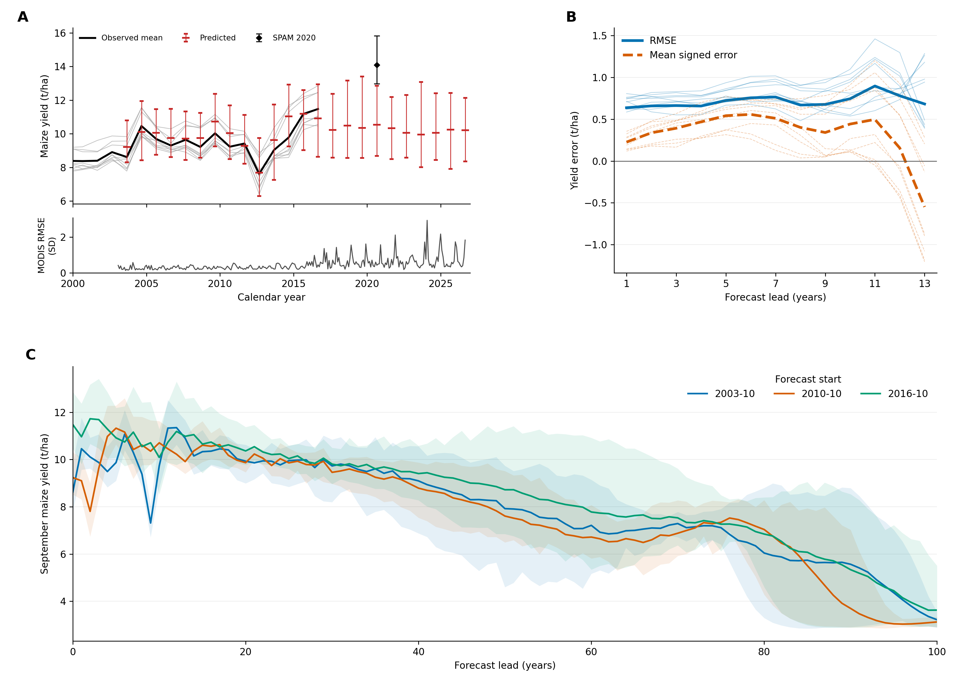
The final figure combines observations, forecast errors, and the century stress test. Download the figure as a PDF.
Candidate pathways
Based on the feasibility assessment summarized below, I propose three candidate pathways for the analysis:
Pathway 1: A global soil carbon transformer, validated with NEON and international flux tower network data.
The model would produce time-series SOC predictions that could then be assessed under climate change scenarios. Global deep-learning SOC models already exist (for example, GSoilCPM), but we have not found one with this kind of temporal validation.
Pathway 2: A hybrid transformer that predicts SOC and crop yield together.
This is a technically difficult pathway. SOC estimates would need to be coarse, probably one pixel per NEON site, so the soil side would be much more thinly constrained than the yield side. The review summarized below suggests a small connection between soil carbon and yield in high-input breadbasket regions but a stronger connection in low-input tropical and dryland systems.
Pathway 3: An autoregressive transformer for cropping-system yields only.
The model would forecast yields by feeding its own output back into subsequent predictions. Suitable data are already identified: yields for four major crops, 1981–2016, at 0.5° (GDHY: The global dataset of historical yields for major crops 1981–2016).
How the idea developed
The project began with two questions. Does a global feed-forward SOC model exist, and could it be tied to food security by identifying SOC concentrations below which particular crops become unsustainable or fail? Five rounds of review followed, each testing the previous version’s assumptions.
Version 1: Initial exploration
Camilo’s initial exploration of the timing of planetary desertification established the modeling background.
CMIP5 and CMIP6 Earth system models simulate soil carbon dynamics, usually as several conceptual pools:
- Turnover times range from months or years (microbial and active litter pools) to centuries or millennia (slow, mineral-associated pools).
- Carbon enters the soil through net primary productivity, as litter, root exudates and dead biomass.
- Carbon leaves as CO₂ and CH₄ through heterotrophic respiration and decomposition.
- Soil temperature and moisture are the main environmental sensitivities, and CMIP6 increasingly includes permafrost physics (Varney et al. 2024; Wei et al. 2022).
Projections of CO₂, temperature, precipitation and SOC feed into global gridded crop models, coordinated mainly through AgMIP.
The initial exploration raised broad claims that had not yet been checked against sources:
- Warming and accelerated SOC mineralization offset CO₂ fertilization gains.
- SOC buffers crops against drought and heat.
- Tropical and subtropical breadbaskets face declining fertility while high latitudes may gain.
Our own takeaway was that SOC thresholds for yield loss or collapse have been proposed but none is agreed upon. The later versions tested these claims directly.
Version 2: Is there an omitted soil-degradation feedback?
The question was reframed as: do global crop-yield projections leave out a soil-degradation feedback, and how large would it be?
The literature search comprised about 120 searches across OpenAlex, Crossref, Semantic Scholar and publisher pages. Nature- and Science-family journals were searched separately, and references were followed from key papers. The resulting bibliography has 183 entries, each with a DOI checked in Crossref; six citations in the starting set needed correcting. Full texts were read in a structured way, and each note records whether it rests on the full text, the abstract or a secondary source.
The review found that the idea is new in scale and method, but not in kind. An “underestimation term” has already been estimated in narrower settings:
- At eight sites, about 4.5 extra percentage points of yield loss at +3 °C (Basso 2018).
- For China, 14% worse losses, though in a stylized scenario where all farmland is set to low quality (Qiao 2022).
- For sub-Saharan Africa, about −24% from declining fertility across 15-16 models (Couëdel 2024, 2026).
- Globally, only in the improvement direction (Deng 2023; He 2025).
There is an identified gap at global scale. The main global crop-model projections, run under the GGCMI phase 3 protocol (Jägermeyr 2021):
- start from soils at equilibrium,
- hold management fixed after 2015,
- leave out erosion,
- and in one model reset soil organic matter every year.
No global, process-based study of degradation’s effect on yield exists, but there is substantial evidence against a large effect:
- Soil carbon adds little to yield once nitrogen is sufficient (Ma 2023). One synthesis found +1.4%, not significant (Hijbeek 2016).
- Soil health explains about 12% of yield variation, against about 70% for management (Xu 2025).
- Benefits seen in field trials do not appear on real farms (Zhao 2026).
- Drought buffering is largest under moderate rather than extreme water shortage (King 2026, contradicting Kane 2021).
- In the strongest test, the soil carbon × climate interaction was small (Couëdel 2026).
The threshold concept is the weakest link. The SOC:clay 1:13 boundary was derived from soil structure in 161 Swiss soils (Johannes 2017) and was never tied to yield. Applied elsewhere, it misclassifies soils: Poeplau and Don (2023) found it labels 94% of German Chernozems as degraded (see also Rabot 2024; Mäkipää 2024; Feeney 2024). It is questionable in tropical soils (Six 2024). Farmers’ perceived thresholds run the opposite way to the ratio, highest in sandy soils (Hijbeek 2017).
Raw CMIP6 soil carbon is unusable for cropland. It includes no management. A modeling artifact also narrows the spread between models (Varney 2022, 2023), and constraining turnover with observations flips the projected 21st-century change from gain to loss (Ren 2024).
The likely result is a small effect in high-input breadbaskets and a more material one in low-input tropical and dryland systems. That points to Nature Food or Nature Communications rather than Science. It also means the transformer baseline must be tested against simpler models.
Version 3: Testing a universal “collapse” floor
A subsequent proposal introduced a universal soil carbon floor of 1–1.2%, combined with CMIP6 soil carbon to date when cropland would cross it, and pitched the result to Science. The assessment found that the factual basis does not hold: no consensus floor exists. Published thresholds range from 1% to 5% soil organic matter, and farmers’ perceived thresholds vary with texture (Hijbeek 2017). Additionally, soils with carbon concentrations below the proposed line were still productive. In England and Wales, 38% of arable sites were already below the “degraded” SOC:clay ratio in 1978–83 and remained productive (Prout 2021).
CMIP6 baseline error is too large. Present-day soil carbon in CMIP6 models spans 514–2913 PgC against about 1561 PgC observed, an error larger than the projected changes.
Crop models are not soil-blind. Several already simulate soil carbon dynamics, which is consistent with Version 2 findings. The models can represent soil carbon, but the global protocol does not let degradation accumulate and affect yield. Two ideas from this round are worth keeping: timing of signal detection (time of emergence) and texture-normalized thresholds. Version 2 shows that the existing texture normalization (SOC:clay) has its own problems, so any texture-based threshold would need a different empirical basis.
Version 4: Boundary review
This round broadened the question: can the systems that feed people lose that capacity, and can production that looks successful hide the loss?
The boundary review considered all 183 references and distinguished source findings from broader inferences and conclusions, recording assumptions, counterevidence, and decisive missing links.
The boundary review found that current yields cannot reveal the long-term condition of the soil producing them. Topsoil can deplete while harvests continue (Evans 2020; Montgomery 2007), and yields and soil condition can diverge (Teng 2024; Laub 2025). Fertilizer genuinely compensates for some constraints (Hijbeek 2016) but not for lost soil depth or compacted rooting zones (Janzen 2006; Alewell 2020). Drought protection is real but is not simply a larger water reservoir. Diverse rotations protected maize under drought, but the water-holding pathways that were measured did not explain why (Renwick 2021). The direct gain in plant-available water per unit of added carbon is modest (Minasny & McBratney 2017). Recovery is slower than prevention. Depleted plots responded poorly to fertilizer and recovered only slowly (Tittonell & Giller 2013). In two of four African trials, carbon and yields declined together (Couëdel 2024, 2026).
The literature’s soil carbon “thresholds” measure different things.
- Soil structure: Johannes 2017; Prout 2021; Rabot 2024.
- Storage ceilings: Georgiou 2022; Heinemann 2024.
- Fertilizer response: Ling 2025.
None is a lower safety limit for food production.
Three routes could turn local losses into a global problem:
- Accumulating local losses (Balkovič 2018).
- Droughts or heatwaves striking several breadbaskets at once (Kornhuber 2023), weighed against evidence that production generally recovers (Lesk 2016).
- Soil–climate coupling, whose sign is uncertain (Varney 2024).
The verdict was that a global, self-reinforcing collapse is unresolved: neither shown nor ruled out. Risk is better judged by three things: the functions that sustain production, the inputs needed to keep those functions going, and how well the system recovers.
Version 5: Historical review of thresholds
The final round asked how food-producing capacity has actually been lost, kept and regained in history, and how soil degradation interacts with climate, water and vegetation.
The existing collection held almost no historical or dryland literature. About 28 outside sources were therefore checked at abstract or summary level only and marked “external,” which lowers confidence in conclusions that rest on them. Each conclusion was labeled Supported, Conditional, Contested or Unresolved.
H1 (Supported): Regions have repeatedly crossed thresholds in their capacity to grow crops. Salinization: southern Mesopotamia (Jacobsen & Adams 1958, contested by Powell 1985) and the Aral basin. Erosion: Mangaia, the Maya lowlands and Iceland (Montgomery 2007). Wind erosion: the Dust Bowl and Kazakhstan’s Virgin Lands. Drought and water loss: the Sahel.
H2 (Supported): The serious crossings shared three ingredients. Each combined slowly lost buffering, a fast climate shock and few alternatives. After the Dust Bowl, migration was the main adjustment (Hornbeck 2012).
H3 (Supported regionally): Land degradation can amplify climate shocks, but not everywhere. Degraded land amplified the Dust Bowl drought (Cook 2009). In the Amazon, rainfall declines once forest loss passes about 25–50% (Leite-Filho 2021). In the Sahel, the ocean was the main driver (Giannini 2003).
H4 (Supported): Losses are hidden beneath stable harvests. About 35% of Corn Belt cropland has lost its topsoil layer, at roughly a 6% yield cost (Thaler 2021). Black-soil topsoil in Northeast China has thinned. The High Plains aquifer is being depleted (Scanlon 2012).
H5 (Supported for drylands, conditional for cropland): Soil fertility drops abruptly at specific aridity levels (Berdugo 2020). This is the strongest genuine soil threshold the reviews found.
H6 (Supported): Soil carbon concentration is not the boundary variable for food production (Zhao 2026; Hijbeek 2026).
H7 (Supported): Large-scale recovery has happened within decades. Farmers regreened over 5 Mha in Niger (Sendzimir 2011). Vegetation in northern Ethiopia is now better than in 1868 photographs (Nyssen 2009). Yellow River sediment from the Loess Plateau fell by about 90% (Wang 2016). Iceland and the North Aral Sea also recovered. By contrast, the Great Green Wall is only about 4% complete in its core zone.
H8 (Conditional): Recovery often shifts limits within the water system rather than removing them (Feng 2016; Cao 2011).
H9 (Conditional): About half of current food production relies on overstepping other planetary boundaries (Gerten 2020; Richardson 2023).
H10 (Unresolved): Whether regional crossings add up to a self-reinforcing global loss remains unresolved.
Synthesis
Across all five rounds, four conclusions hold:
- No universal soil carbon threshold for yield exists.
- Raw CMIP6 soil carbon cannot drive the study.
- Current harvests do not prove soils are healthy.
- Any soil effect omitted from global projections is likely concentrated in low-input tropical and dryland systems.
Together, these move the question from “when will soil carbon cross a collapse threshold?” to “where is soil decline eroding production capacity in ways yields do not yet show?”
Transformer feasibility experiment
Objective and outcome
This experiment adapted an existing transformer to jointly predict monthly MODIS observations and maize yield, then tested how its forecasts behave when repeatedly fed back as inputs. The work progressed from aligning global datasets, through a small comparison of two training approaches, to a larger autoregressive training run and an evaluation on nine previously unused Iowa pixels.
After 15 epochs, the larger model achieved 0.689 t/ha RMSE at the next annual yield anchor, compared with 1.160 t/ha for persistence, a 40.7% reduction. The separate Iowa evaluation showed partial cancellation of errors when pixels were averaged, underprediction relative to a 2020 SPAM yield reference, and substantial downward drift during century-long rollouts. These results support short-horizon predictive skill in the tested setting while exposing limitations in continued autoregression.
1. Source data and preparation
Two yield datasets were organized and reviewed: GDHY for annual historical yields and SPAM 2020 for a finer-resolution spatial reference. Original downloads were retained separately from the derived rasters and samples.
| Dataset | Coverage used or available | Role |
|---|---|---|
| GDHY aligned v1.2 and v1.3 | Annual, 1981–2016; 0.5° grid | Historical maize yield labels |
| SPAM 2020 | 2020 snapshot; 5 arc-minute grid | Separate yield spot check beyond GDHY coverage |
| MODIS MOD09CMG Collection 6.1 | Monthly exports from February 2000 through October 2026 | Spectral and thermal predictors and targets |
GDHY NetCDF rasters were converted to GeoTIFFs for consistent GIS display and subsequent extraction. The working grid is EPSG:4326, 720 columns × 360 rows, with 0.5° cells, spanning −180° to 180° longitude and −90° to 90° latitude. Correcting the source longitude convention and preserving row orientation resolved the original display/alignment problem. Monthly imagery was requested on this same grid, and raster dimensions, transforms, and coordinate systems were checked for exact agreement.
Initial imagery work included Landsat, but the sustained pull moved to coarser products to reduce extraction cost. The monthly export workflow covered MODIS, AVHRR, TerraClimate, and CFSv2, with Landsat and Dynamic World omitted from that pull. Only MODIS, yield, and calendar features entered this modeling experiment. The other products were not combined with MODIS or treated as interchangeable sensors.
Monthly arithmetic means were submitted as Earth Engine batch tasks, staged as Earth Engine assets, and downloaded locally. No Google Drive export was used. Polar footprint transformation failures were handled by staging the interior rows and retrieving the two polar rows separately on the same grid, averaging their source observations locally. The resulting files retained the full global grid. This was a direct coarse-grid export workflow, not an explicit fine-resolution, area-weighted reconstruction of every output cell.
The exports retained all supplied bands, but the model selected seven surface-reflectance bands and four brightness-temperature bands (20, 21, 31, and 32). No additional cloud filtering was applied. Monthly averaging was the temporal aggregation; no further spectral smoothing was introduced. October 2026 was excluded from the final evaluation because it was incomplete. The yield references are GDHY and SPAM 2020.
2. Monthly yield representation and model
Annual GDHY yields, in tonnes per hectare, were converted to a monthly sequence by linear interpolation between annual anchors: September 1 in the northern hemisphere and March 1 in the southern hemisphere. At an anchor, the monthly value equals the original annual yield. Between anchors, it gradually changes from that year's value toward the following year's value, weighted by elapsed time. These monthly values are smoothed labels, not independent monthly harvest measurements.
Each input consisted of the preceding 36 months, with 14 features per month: 11 MODIS values, maize yield, and sine/cosine encodings of calendar month. Feature means and standard deviations were calculated from training pixels only. Yield was both an input and an output.
The existing soil-carbon and fire-weather frameworks informed the setup. The implemented model definition was copied unchanged from the original fire-weather notebook: a linear embedding to 256 dimensions, sinusoidal positional encoding, six transformer encoder layers, eight attention heads, and dropout of 0.1. Three learned queries pool the encoded sequence into three output heads, configured here to return 11 MODIS values, one yield value, and two calendar features. These are three pooling queries within one model, not three separate forecasts.
Two training approaches used this same architecture:
- Standard: predict the next monthly row and minimize mean squared error on that row.
- Autoregressive: predict 12 successive rows, repeatedly appending predicted MODIS and yield to the rolling history. Known calendar values are supplied at each step. Loss covers all 12 steps, and gradients propagate through the feedback sequence.
Loss was calculated across all 14 standardized outputs, including the calendar head. During rollout, the known calendar replaces its predicted counterpart before feedback. Training used Adam with learning rate 0.0001 and random seed 42. Both pilot models started from the same initialization. Training and forecast inference ran on the AMD Radeon 8060S GPU; no CPU training was used.
3. Pilot experiment
The pilot used 16 pixels, balanced between hemispheres: 12 training pixels and four validation pixels. Both training approaches ran for two epochs. A stride of 13 months produced 144 training windows and 48 validation windows while varying the starting season.
| Pilot yield evaluation | Standard RMSE | Autoregressive RMSE |
|---|---|---|
| Next month | 3.892 t/ha | 1.504 t/ha |
| Across a 12-month rollout | 4.122 t/ha | 1.537 t/ha |
Autoregressive training performed better than standard training in this small pilot, but persistence achieved 0.390 t/ha over the monthly rollout. The pilot therefore established that the training and feedback paths worked; it did not establish superiority to a simple baseline.
A 36-month forward run demonstrated that the model could continue beyond its 12-month training horizon. Historical backtests then used ten annual origins at each of the four validation pixels. Yield RMSE at one, two, and three years was 1.525, 1.604, and 1.745 t/ha, respectively; persistence achieved 0.772, 0.949, and 0.965 t/ha. None of the 11 MODIS bands beat repeating the preceding year's seasonal cycle in that pilot backtest. These findings motivated the larger run and explicit scoring at annual yield anchors.
4. Expanded training and coverage audit
The larger sample contained 1,000 pixels, with 500 in each hemisphere. Whole pixels were split into 750 training and 250 validation pixels, rather than splitting windows from the same pixel across those sets. All selected locations had complete annual yield records for 1999–2016 and complete MODIS histories for the training period, February 2000–March 2016: 194 monthly rows per pixel.
This represented about 9.0% of the 11,119 locations with complete maize yield records; training alone used 6.7%. That denominator is the complete-yield pool before checking global MODIS completeness, not the whole global grid or the full area where maize is grown.
A separate coverage audit examined whether pixels appeared to enter or leave maize production. Of 15,113 locations with any GDHY maize coverage during 2000–2016, 3,994 had missing years. GDHY's fixed crop geography around 2000 means these gaps cannot be interpreted as planting changes. Zero yield was retained as a valid label and distinguished from missing data. Twenty training pixels and three validation pixels had at least one zero-yield year. The audit was recorded without changing the ongoing training design.
The larger run used a one-month window stride, batch size 64, 110,250 training windows, and 36,750 monthly validation windows. A separate set of 3,125 annual-anchor validation windows started at known annual yields and ended at the following annual anchor. The best checkpoint was selected by that annual-anchor error. A basic local dashboard displayed training logs and metrics.
Autoregressive training was paused at the saved epoch-15 checkpoint. An unfinished portion of epoch 16 was discarded. The larger standard-model run had not started, so there is no full-scale standard-versus-autoregressive comparison. The 15 completed epochs took approximately 9.38 hours, averaging 37.5 minutes each.
| Yield metric | Epoch 1 | Epoch 15 | Persistence |
|---|---|---|---|
| Training rollout RMSE | 0.792 | 0.330 | — |
| Validation next-month RMSE | 0.663 | 0.327 | — |
| Validation 12-month rollout RMSE | 0.775 | 0.458 | 0.516 |
| Validation next annual-anchor RMSE | 1.088 | 0.689 | 1.160 |
All values are in t/ha. Training RMSE aggregates batches while weights are changing; it is not a fixed-checkpoint evaluation of the training set. Persistence holds the latest input yield constant. At epoch 15, monthly rollout RMSE was 11.1% lower than persistence and annual-anchor RMSE was 40.7% lower.
Monthly training and validation windows were constructed from the full interpolated yield series. Consequently, an input between annual anchors can already incorporate part of the next annual label. Annual-anchor validation avoids that particular issue. The later Iowa forecasts also explicitly prevented future annual labels from entering their seeds.
5. Separate Iowa evaluation
A contiguous 3 × 3 block in central/eastern Iowa, centered at 42.25°N, 92.75°W, was selected for geographic suitability and complete records. The block spans 41.5–43.0°N and 93.5–92.0°W. None of its nine pixels occurred in either the pilot or larger training/validation samples. It was selected before computing its forecast scores.
The unchanged epoch-15 model was evaluated from 165 monthly starting dates, February 2003 through October 2016. Every start used 36 observed months. Only annual yield anchors available by the final observed month were permitted in that seed; after the latest available anchor, its yield was held constant. This prevented the interpolated input from revealing the next year's yield. Subsequent steps fed back predicted MODIS and yield, with only the calendar supplied externally.
Yield forecasts were compared with GDHY through September 2016. MODIS forecasts could be evaluated much further, through September 2026. SPAM supplied a separate September 2020 yield spot check. Each model cell contains 36 SPAM cells, giving 324 finer pixels across the Iowa block. SPAM values were converted from kg/ha to t/ha. Arithmetic spatial means were used; matching harvested-area weights were not available.
Signed error was defined as prediction minus reference. Positive values indicate overprediction; negative values indicate underprediction. RMSE measures error magnitude without preserving its sign. Individual-pixel scores were calculated across eligible starts at each forecast lead. For group scores, the nine forecasts and nine references were first averaged spatially, then compared. Thus the group RMSE measures error in the mean forecast, not the arithmetic mean of nine RMSEs. The model still predicts pixels independently; this tests spatial error cancellation, not a coupled pixel network.
6. Forecast results and interpretation
| Yield lead | Eligible starts | Pooled individual RMSE | Group-mean RMSE | Group signed error |
|---|---|---|---|---|
| 1 year | 153 | 0.705 | 0.637 | +0.226 |
| 5 years | 105 | 0.798 | 0.723 | +0.542 |
| 10 years | 45 | 0.843 | 0.745 | +0.442 |
| 13 years | 9 | 0.897 | 0.682 | −0.549 |
Errors are in t/ha. Averaging reduced yield RMSE, but it did not remove systematic error. The number and calendar distribution of eligible starts change with lead time. In particular, the lower group RMSE and negative bias at 13 years rely on just nine starts and do not establish that forecasts improve with age. Overlapping starts and neighboring pixels are not independent replicates.
Across the 324 finer SPAM pixels, the 2020 mean was 14.09 t/ha, with values from 12.98 to 15.83 t/ha. The mean September 2020 prediction across all eligible starts and nine model pixels was 10.54 t/ha. Depending on start date, RMSE against the nine coarse-cell SPAM means ranged from 2.82 to 4.22 t/ha. This spot check shows underprediction relative to SPAM, but differences between SPAM and GDHY methodologies and spatial weighting prevent attributing the entire discrepancy to temporal drift.
MODIS error increased over longer leads: pooled standardized RMSE was 0.365 at one year, 0.701 at ten years, and 0.867 at sixteen years. Averaging the nine pixels reduced those errors by about 14.1%, 6.1%, and 4.3%, respectively. Recurrent winter error peaks were visible across forecast starts. Clouds are a plausible contributor, alongside snow and seasonal variation; that attribution was not tested. The exploratory analysis retained the MODIS signal as supplied, including possible cloud effects.
Finally, three fixed starts—October 2003, October 2010, and October 2016—were each advanced 1,200 months, with no observations, clipping, or resets during the rollout. All remained finite and all developed downward yield drift. Their nine-pixel mean September yields at year 100 were 3.22, 3.12, and 3.62 t/ha, respectively. These trajectories describe the model's long-run behavior, not an established century-scale agricultural trend.
The evaluation holds out pixels, not the historical calendar period: training pixels cover many of the same years as the test histories. Nearby training pixels may also share regional conditions. GDHY and SPAM are modeled yield references, and monthly GDHY values are interpolated annual labels. RMSE, pixel ranges, and variation across starts are not calibrated predictive uncertainty intervals. The century experiment demonstrates that good one-year validation does not guarantee stable long-run autoregression.
Meetings and notes
I met with Robert Kennedy and the LandTrendr team, who expressed interest in the concept. One possibility is for the Kennedy lab to provide computing resources for our model runs; another is to develop a broader collaboration. These are possibilities to explore, rather than arrangements already in place. My concern is that organizing a collaboration could slow progress, so I would want to understand what it adds and how it affects the timeline.
I also met with Corey Scher. One direction that emerged is to incorporate conflict into the framework, alongside changes in ecosystems and agricultural production. The broader question is: “What is going to kill us first, ecosystem collapse or conflict?” This would extend the work to consider how conflict disrupts agriculture, and how those disruptions interact with environmental change.
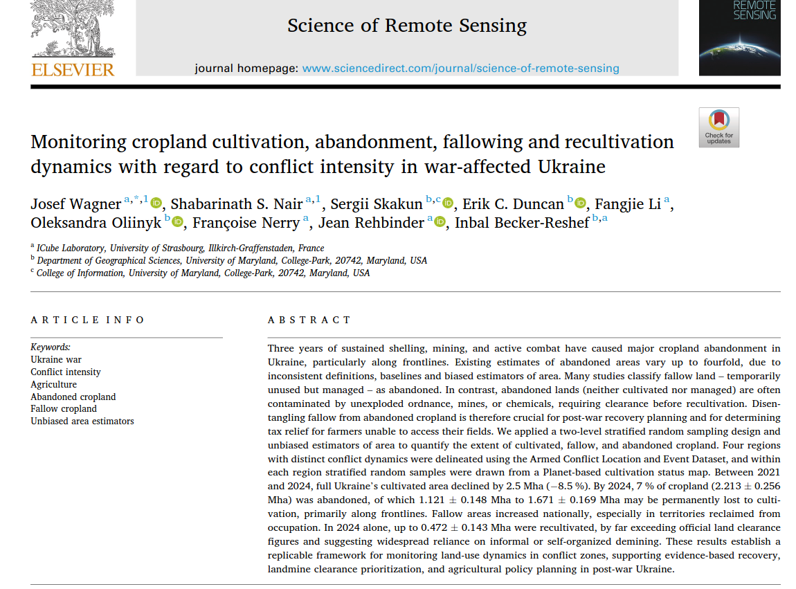
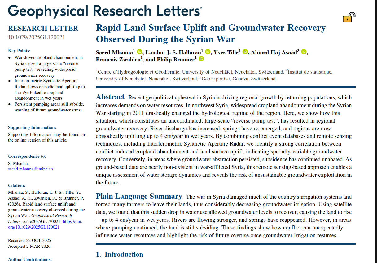
In our exchange, Corey suggested ACLED conflict events, aggregated to administrative units, as a possible covariate. He also mentioned agricultural-damage benchmark data being assembled for a NASA project, although those data are unlikely to extend much earlier than the Sentinel-2 period. The paper excerpts below offer two examples of the connection: changes in cropland use in Ukraine, and groundwater recovery following reduced irrigation during the Syrian war.